
Learning Graph Structures, Graphical Lasso and Its Applications - Part 3: Inverse Covariance Matrix and Graph
Published:
Let us look at one hypothetical undirected graph:
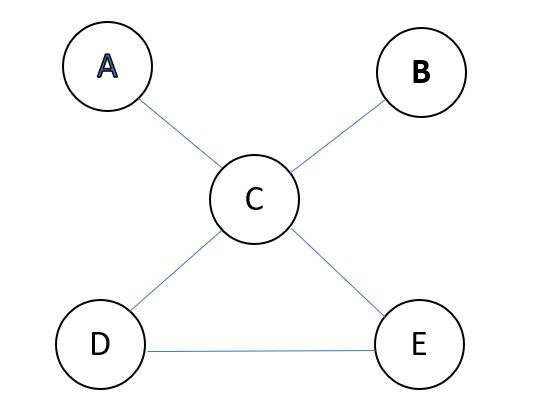
Let us focus on vertices A and B, and their neighbor C, we have their joint distribution P(A, B, C), right?
By the property of undirected graph or Markov Field more formally, this can be decomposed as P(A,B,C) = P(A,B|C)P(C) = P(A|C)P(B|C)P(C), which says A and B are conditionally independent given C. In an undirected graph, if C blocks A and B, then A and B are conditionally independent given C. Note that we naturally have P(A,B,C,D,E) = P(A|C,D,E)P(B|C,D,E)P(C,D,E) too, as C, D and E can be seen as blocking A and B together.
Now, what does conditionally independent variables say about the inverse covariance matrix?
Let me state the conclusion here first: we can show that two variables conditionally indepedent given all other variables in the graph correspond to a value of 0 in the corresponding cell in the inverse covariance matrix.
First of all, let us remind ourselves of the conditional gaussian distribution:
Take our Np data matrix as example again. Each data point is of p dimensions, which could be split into two components with a and b dimensions each and a+b=p. For example, if we originally have a vector X ( \(X_{1}\), \(X_{2}\), ..., \(X_{a}\) ), we could, say, treat the first a elements as belonging to the first component, and the rest, namely, ( \(X_{a+1}\), \(X_{a+2}\), ..., \(X_{p}\) ) as belonging to the second. It follows the gaussian distribution parameters will be: $$\begin{array}{c}{\mu=\left( \begin{array}{c}{\mu_{A}} \\ {\mu_{B}}\end{array}\right)} \\ {\Sigma=\left( \begin{array}{cc}{\Sigma_{A A}} & {\Sigma_{A B}} \\ {\Sigma_{B A}} & {\Sigma_{B B}}\end{array}\right)}\end{array}.$$ Now, the conditional distribution of \(X_{A}\) given \(X_{B}\) = \(x_{B}\) will be in the form: $$N\left(\mu_{A|B}, \Sigma_{A | B}\right) \text { where } \mu_{A | B}=\mu_{A}+\Sigma_{A B} \Sigma_{B B}^{-1}\left(x_{B}-\mu_{B}\right) \text { and } \Sigma_{A | B}=\Sigma_{A B}-\Sigma_{A B} \Sigma_{B B}^{-1} \Sigma_{B A}.$$ Note from the form of the conditional mean that if A is independent of B then Cov(A,B) =0 and vice versa, which means the covariance matrix is diagonal. Similarly, consider picking two dimensions i and j from the set A, and given all other dimensions as known, the sub-covariance matrix for i and j will be diagonal too: $$\left( \begin{array}{cc}{V a r_{i}} & {\operatorname{Cov}_{i j}=0} \\ {\operatorname{Cov}_{j i}=0} & {\operatorname{Var}_{j}}\end{array}\right).$$And of course, the inverse of a diagonal matrix is also diagonal. Now we have shown that if two dimensions i and j are conditionally independent given all other dimensions, the corresponding term in the inverse covariance matrix will be 0.
Equipped with all these assumptions and facts, we are now ready to tackle the problem of estimating the inverse covariance matrix.
Before diving into a clever solution of this problem, let me state one more practical assumption, which is that the inverse covariance matrix is sparse, which means that there are lots of conditionally independent pairs of variables in our graph and that there are lots of zeros in the inverse covariance matrix.
This actually makes sense, as in practice we may as well set some thresholds to filter out the weak edges.
Now we are all set and let us go to the solution of the problem.