
Learning Graph Structures, Graphical Lasso and Its Applications - Part 8: Visualizing International ETF Market Structure
Published:
I will try to illustrate the power of graphical lasso with an example which extracts the co-varying structure in historical data for international ETFs. This experiment shows some interesting patterns which can be exploited for constructing more complex models in pairs trading, building hedging portfolios, etc.
Specifically, the inverse covariance matrix inferred by graphical lasso corresponds to how different ETFs correlate conditionally on the others. In the graph, each node, marked by the country name, represents an ETF ticker, and is connected to those that potentially explain its fluctuations in historical returns.
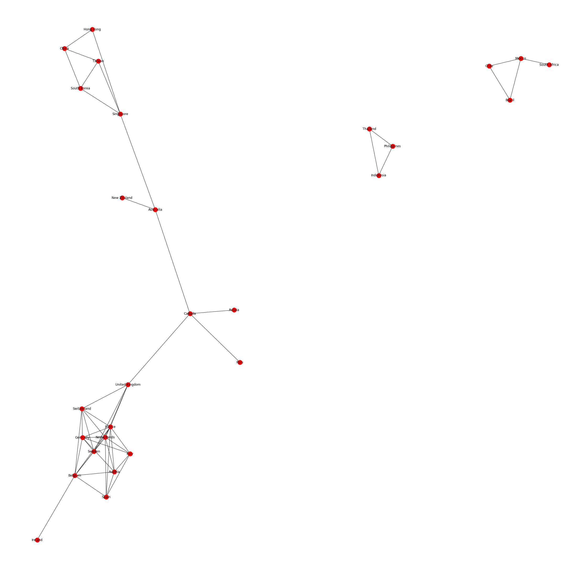
The following Python snippet can be used as a starting point for replicating the graph above and for other interesting data explorations. The readers are encouraged to tweak the different options and be imaginative in their own projects.
import pandas as pd
import matplotlib.pyplot as plt
from sklearn import covariance
import numpy as np
import networkx as nx

#Setting up the mapping from ticker to country
#To be specific, we collected the daily closing price series between 04/11/2011 and 04/10/2019 from Yahoo Finance:
etfs = {"EWJ":"Japan","EWZ":"Brazil","FXI":"China","EWY":"South Korea",
"EWT":"Taiwan","EWH":"Hong Kong","EWC":"Canada","EWG":"Germany",
"EWU":"United Kingdom","EWA":"Australia","EWW":"Mexico","EWL":"Switzerland",
"EWP":"Spain","EWQ":"France","EIDO":"Indonesia","ERUS":"Russia","EWS":"Singapore",
"EWM":"Malaysia","EZA":"South Africa","THD":"Thailand",
"ECH":"Chile","EWI":"Italy","TUR":"Turkey","EPOL":"Poland","EPHE":"Philippines",
"EWD":"Sweden","EWN":"Netherlands","EPU":"Peru","ENZL":"New Zealand",
"EIS":"Israel","EWO":"Austria","EIRL":"Ireland","EWK":"Belgium"}
symbols, names = np.array(sorted(etfs.items())).T

#Read in series of daily closing prices
#The file 'input.csv' uses the tickers above as columns, and dates as index in df
df = pd.read_csv("input.csv")
del df['Date']

#Convert price series to log return series
df = np.log1p(df.pct_change()).iloc[1:]

#Prepare the list of countries in the same order as the input columns
cols = df.columns
ctries = [etfs[c] for c in cols]
cols = pd.Series(ctries)

#Calling Glasso algorithm
edge_model = covariance.GraphicalLassoCV(cv=10)
df /= df.std(axis=0)
edge_model.fit(df)
#the precision(inverse covariance) matrix that we want
p = edge_model.precision_

#prepare the matrix for network illustration
p = pd.DataFrame(p, columns=cols, index=cols)
links = p.stack().reset_index()
links.columns = ['var1', 'var2','value']
links=links.loc[ (abs(links['value']) > 0.17) &  (links['var1'] != links['var2']) ]

#build the graph using networkx lib
G=nx.from_pandas_edgelist(links,'var1','var2', create_using=nx.Graph())
pos = nx.spring_layout(G, k=0.2*1/np.sqrt(len(G.nodes())), iterations=20)
plt.figure(3, figsize=(30, 30))
nx.draw(G, pos=pos)
nx.draw_networkx_labels(G, pos=pos)
plt.show()
References:
Goto, S., Xu, Y.: Improving mean variance optimization through sparse hedgingrestrictions. Journal of Financial and Quantitative Analysis 50(6), 14151441 (2015)
Stevens, G. (1998). “On the inverse of the covariance matrix in portfolio analysis.” The Journal of Finance, 53: 1821–1827.